PINNs Part 1: Existing Work

PINNs: physics informed neural networks

Maziar Raissi, Paris Perdikaris, and George Em Karniadakis introduced the physics informed neural network (PINN) in this 2017 paper. The PINN is a neural network trained to solve general nonlinear partial differential equations in a semi-supervised manner while respecting physical laws. This writeup details my understanding and Python implementation of some of the work presented in the paper. I go on to apply the techniques introduced in this paper to a new problem in part 2. A basic understanding of the fundamentals of neural networks, calculus, and differential equations is assumed.

There are many different methods used to find analytical solutions of PDEs, but not all PDEs can be solved (at least, there are many PDEs that nobody has solved yet). This is where approximation methods come in to help. For these hard-to-solve PDEs, several different numerical methods exist that can be used to approximate their solutions with sufficient accuracy. The PINNs paper focuses on training neural networks to approximate the solutions of PDEs that describe physical systems instead of using traditional numerical methods.

Burgers' equation

The paper begins by applying a PINN to solve Burgers' equation in one spatial dimension:

for $x \in [-1, 1]$ and $t \in [0, 1]$ with initial and boundary conditions:

The paper defines the left-hand side of the PDE as:

The goal is to train a neural network to predict the solution to the PDE, $\hat{u}$, from inputs $x$ and $t$ while considering the constraints applied to the system by the boundary/initial conditions and $f$.

We know what the value of $\hat{u}$ should be at $t=0$, $x=-1$, and $x=1$. As I understand it, the paper seems to define collocation data as values of $x$ and $t$ that lie within their respective domains, but do NOT sit on these boundary/initial conditions. For these collocation values of $x$ and $t$, all we know is that $\hat{u}$ should satisfy Burgers' equation (this is quantified by the expectation that $f=0$).

Neural networks are differentiable functions, which means that we can compute the gradient of $\hat{u}$ with respect to each input $x$ and $t$ (i.e. we can find $\hat{u}_x$, $\hat{u}_{xx}$, $\hat{u}_{t}$), which gives us the remaining pieces we need to calculate $f$ for a prediction. This is made possible by the automatic differentiation features implemented in Tensorflow and PyTorch.

To train this network, we need data. The data is created by generating pairs of random $x$ and $t$ values in their respective domains (excluding the boundary values $t=0$, $x=-1$, $x=1$). The paper uses latin hypercube sampling for data generation, but I instead sample from uniform distributions for simplicity's sake. For each of the three boundary conditions, data is generated by fixing either $x$ or $t$ and random sampling the other value. Meaning, set $t=0$ and then generate random $x$ values, then set $x=-1$ and generate random $t$ values, then set $x=1$ and generate random $t$ values.

For the boundary/initial condition data, $\hat{u}$ is directly compared to its expected value. For the non-boundary/initial condition data, $f$ is found and compared to its expected value, $0$.

The loss of the network is defined as:

where

and

Since the expected $f$ is always equal to $0$, $MSE_f$ simplifies to:

$MSE_u$ basically says "for a set of $x$ and $t$ boundary/initial condition data, how far off are the predictions $\hat{u}$ from the known values of $u$, on average?"

$MSE_f$ basically says "for a set of $x$ and $t$ that are NOT boundary/initial conditions, how well do the predictions $\hat{u}$ satisfy Burgers' equation, on average?"

Extending from there, $MSE$ says "for a set of $x$ and $t$ that contains boundary/initial condition data and non-boundary/initial condition data, how well do the predictions $\hat{u}$ satisfy the boundary/initial conditions and Burgers' equation, on average?"

The closer the network's predictions are to correct, the closer $MSE$ is to 0. So, the goal of the PINN is to minimize $MSE$. These loss criteria are what drive the PINN to make predictions that are constrained to the physical definition of the PDE.

Code implementation

The code referenced in the paper uses Tensorflow, but I prefer PyTorch. The complete Python notebook I developed can be found here. I display and explain snippets of this notebook below.

The following function generates boundary, initial condition, and collocation data. It then splits all of the data into train/test sets for modeling.

That's a lot of logic to digest, but the above code basically generates data for the $t=0$, $x=-1$, $x=1$ cases and collocation cases. The paper uses $N_u=100$ and $N_f=10000$, a proportion $N_u/N_f = 0.001$. I assume that the $N_u=100$ samples are split evenly between the cases $t=0$, $x=-1$, and $x=1$, meaning that the proportion of each boundary/initial set of data to $N_f$ is approximately $0.0003$. The actual values of $N_u$ and $N_f$ I use are slightly different than the paper, but the proportions of data split are the same.

Now, let's define the PINN and its associated loss:

The paper uses a feed-forward neural network with 9 dense layers containing 20 neurons and hyperbolic tangent activation functions. This seems like a somewhat arbitrary choice of architecture to me, but it's simple and it works.

The trickiest part of the above code is the PyTorch gradient calculation (lines 71-73), as it took me a while to figure out the correct syntax for the autograd.grad() function. Typically when you train a neural network with PyTorch, you don't explicitly call this function, but, in order to calculate the gradients of $\hat{u}$ with respect to the inputs $x$ and $t$, this is necesssary. The unique usage of automatic differentiation is the most clever part of the PINN, in my opinion. The rest of the code presented above is fairly boilerplate PyTorch neural network code.

Alright, now let's train the model on the generated data. First, the data must be split into batches. It's usually more computationally efficient to pass batches of data through the neural network rather than a single sample at a time, especially when utilizing a GPU. The network also learns better if the loss is calculated based on the mean loss of multiple samples rather than a single sample. Batching the data is an easy reshape:

With the data in batches, the training loop is defined:

Each forward pass in the training loop above consists of passing a batch of boundary and initial data through the network and then passing a batch of collocation data through. $MSE_u$, $MSE_f$, and then $MSE$ are calculated. Next, the network backpropagates from $MSE$ and updates its weights and biases. After all batches of data have been forward and backward passed through the network, mean train loss values are calculated, and then the test data is passed through the network and its loss values are calculated. These steps are repeated num_epochs times.

Results

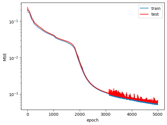
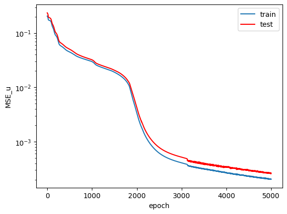
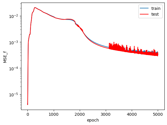
The paper doesn't appear to mention the number of training steps or epochs used to attain the results presented, so I trained a few networks on different numbers of epochs and batch sizes. After a few experiments, I settled on using a dataset of $N=100000$ and training on $5000$ epochs. The mean train and test $MSE$, $MSE_u$, and $MSE_f$ values appear to converge to "stable" and "small enough" values. Although I didn't use the exact $N$ used in the paper, data generation for this problem is relatively cheap, and I really just wanted to see if I could get a network to learn the problem with a decent level accuracy.

The loss plots across the training epochs:

$MSE_f$ starts at a very low value on the order of $10^{-5}$ and then quickly increases before finally converging to a value on the order of $10^{-3}$. I believe the initial loss value was so low because the network learned to predict $\hat{u}=0$ first, which would have led to a very low value of $f$. $MSE_u$ on the other hand, shows a more consistently decreasing trend across training. Following my guess about the network initially predicting $\hat{u}=0$, I expect that the relatively large $MSE_{u}$ value in the early training epochs (compared to $MSE_f$) led the network away from predicting the trivial solution and pushed it towards making predicitons that satisfy both loss terms appropriately. Admittedly, this network could have probably seen slightly better convergence had it been trained for more epochs. I don't see much of an overfit on the train data when compared to the test data, which suggests that the model learned to predict a general solution that not only applies to the specific data it has seen.

Another interesting feature to note is the erratic sort of behavior near the end of training in the $MSE_f$ term. It seems odd that this behavior only started later in training while the curve looked smooth beforehand. My gut response is to say "oh that's some sort of numerical instability thing," but that doesn't feel like a satisfactory answer. It seems to me that once the model converged to a "good enough" solution, slight tweaks in its weights and biases somehow led to large changes in the calculation of $f$. This is only speculation, as I would need to analyze how the gradients $u_x$, $u_{xx}$, and $u_t$ vary based on the value they're differentiated with respect to in order to confirm my suspiscions.

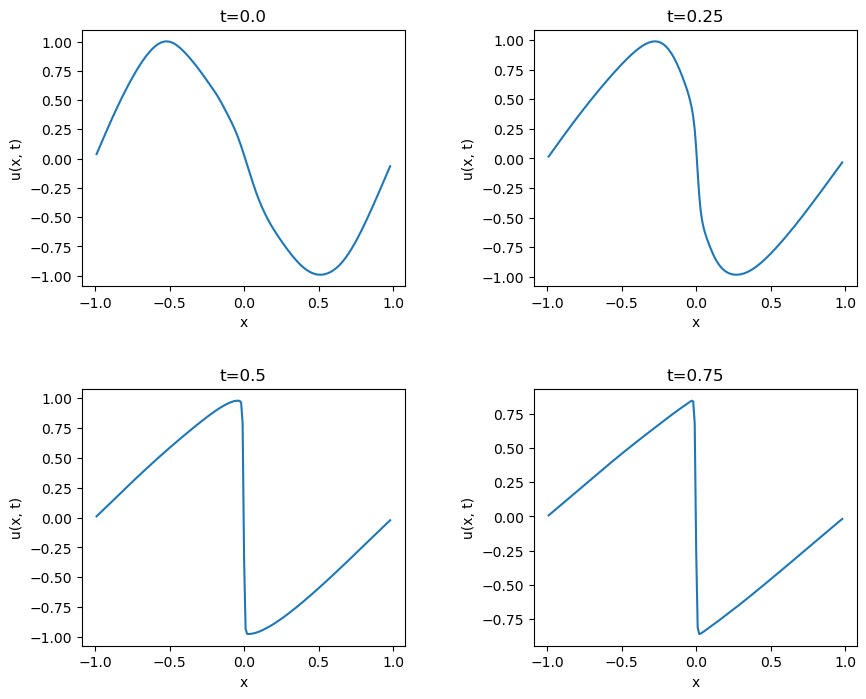
The predictions of $u$ across all $x$ at four snapshots in time:

Qualitatively, the predicted $u$ values at each time snapshot look very similar to the exact results displayed in the paper. The shape of $u$ across all $x$ takes on the expected distribution which initially looks like a sinusoid and then progressively approaches a sawtooth-looking shape with a steep drop at $x=0$. The model learned to predict the $t=0$, $x=-1$, and $x=1$ conditions very well. The paper cites this as a source that contains the analytical solution to this version of Burgers' equation. The solution looks quite non-trivial to understand and implement (and I'm not that interested in doing so), so I'm unable to quantify the L2 error in my network's predicitons like the paper does. It pains me to not generate this metric for comparison, but my implementation appears to work, and I'd like to move on to new applications of PINNs.

While experimenting, I removed the $MSE_u$ term to see if the model would still learn to satisfy Burgers' equation using only $MSE_f$. The resulting model predicted a constant value of about $-0.15$ across all $x$ for all $t$. I really don't know why it learned to do that, but I've read that physics-informed machine learning methods have issues with stability and loss convergence when they aren't properly constrained, and this behavior is a great example of the sensitivity of PINNs.

Next steps

The paper goes on to apply the PINN approach to other PDEs and discusses variations to the approach and their results. I'm convinced that I understand enough about PINNs now and am moving on to part 2 where I apply the techniques discussed herein to a harder problem. See you there.