Transformers - Part 1: Theory

I'd like to start out by saying that I've known about transformers since GPT 1. I'm not one of these new-age LLM hype guys, but ChatGPT and other LLMs are here to ruin us all, so I decided I might as well understand them.

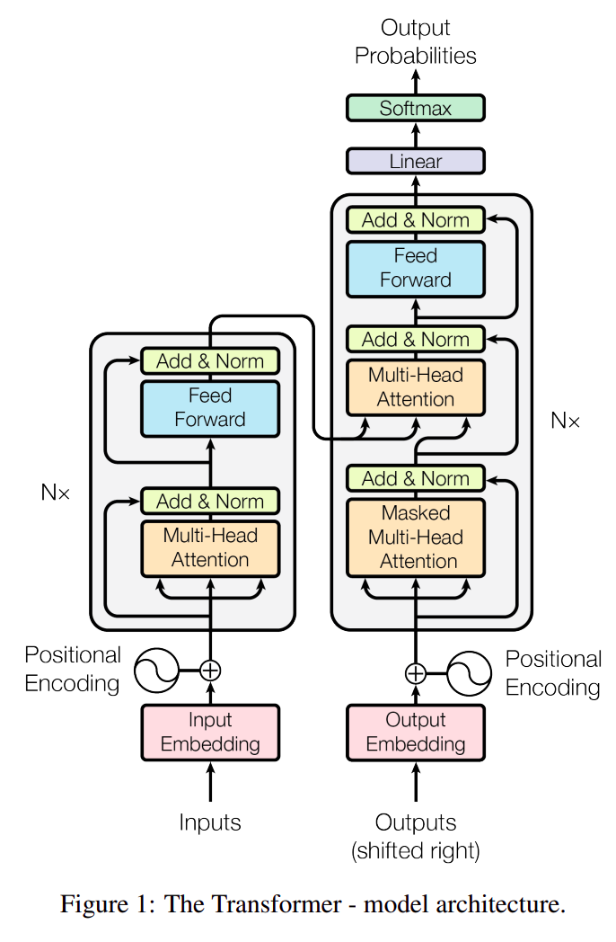
The transformer neural network architecture was first proposed in 2017 in the paper "Attention is all you need" (arXiv link). This is the core architecture that GPT models are based on (although we can't know the details because OpenAI has to keep us safe by not open sourcing anything). The rest of this post details my interpretation of the transformer architecture described in the paper. I work through each piece of the architecture in the diagram below in the most logical beginning-to-end order I have thought of.

Inputs and outputs

The paper seems to assume your inputs are some generically-defined sequential data. The authors tested their architecture on an english-german translation task, so I decided to base my understanding off of an english-spanish translation task (I chose spanish because I'm familiar with its basic grammatical structure and vocabulary).

A single sample of an english-spanish translation dataset might look like:

english	spanish
"He is tall."	"El es alto."

I don't want to get too caught up on the specific data used, since I'm just focused on understanding the transformer architecture, but I will refer to this type of data when explicit examples are needed.

Input and output embedding

The sentence strings must be converted into numeric representations in order to be passed into the transformer. First, the sentence strings must be broken down into individual tokens. The set of unique tokens across all sentences in the training data makes up the vocabulary for each language. Once the sentences are tokenized, each token must be mapped to a fixed-length vector. The values in these fixed-length vectors can either be learned with an embedding layer in the neural network, or pretrained values can be used.

Let's say we have a model or layer that allows for a mapping of a token to a vector. With this, we can map each token in each sentence to a fixed-length vector. Stack those vector representations on top of each other, and boom, you've got an input matrix for the transformer. This is great, but, the sentences in our data will probably vary in the number of tokens contained. The transformer (like every other neural network) needs a fixed input shape. The solution is to simply pad the input matrices with rows of 0s. This puts a maximum on the number of tokens that an input sequence can have, but it also allows for "variable" length inputs, so long as the length is less than the maximum allowed.

Let's use the sentence "He is tall." as an example. We apply whatever language-specific rules we've come up with and split this string into 4 tokens:

["He", "is", "tall", "."]

In addition to the actual tokens in the sequence, we must add special start and end tokens "<S>" and "<E>" (reasoning explained later), which makes our input:

["<S>", "He", "is", "tall", ".", "<E>"]

We then use our token-to-vector mapping to map these tokens to vector representations. Let's say our model maps the tokens to vectors of length 5. I'm making all of these numbers up, but let's say the input tokens map to the following vectors:

Let's set the maximum number of tokens in a sentence to 8. After padding the data with rows of 0s, the input sequence maps to the matrix:

Moving forward, it will be useful to have a consistent definition of our variables:

• embedding_len: size of one embedded input vector
• num_tokens: maximum number of tokens in a sequence

In the example above, embedding_len = 5 and num_tokens = 8.

Positional encoding

In order to give each embedded token vector information about its position in the sequence, the paper presents the following equations:

Where $pos$ is the row index of the sequence matrix, $i$ is the dimension, and $d_{model}$ is the dimensionality of the input (i.e. num_tokens * embedding_len). The first equation with $sin$ is used to get a positional encoding for even indices in the token vector, while the $cos$ equation is used for odd indices.

Given a sinusoid function $sin(cx)$ where $c$ is a constant, the wavelength (peak-to-peak distance) is given by:

For $PE$, when $pos$ attains its minimum value of $0$, the wavelength attains a minimum of $\lambda=2 \pi$. For any other value of $pos$, when $i=0$, the wavelength attains a maximum of $\lambda=10000*2 \pi$. This scheme allows each word vector in an embedded sentence matrix to have a unique set of positional values.

A quick visualization of the differing frequencies of $PE$ shows the progression of positional encoding values:

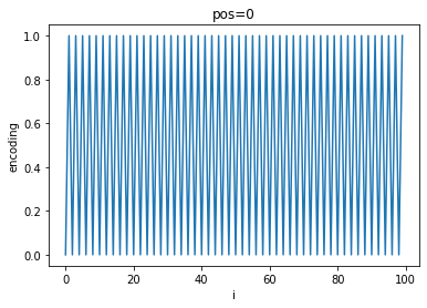
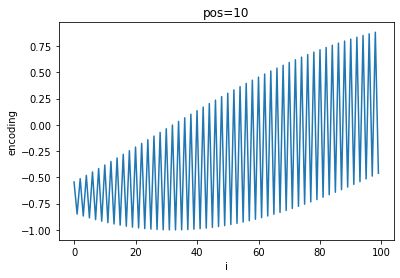
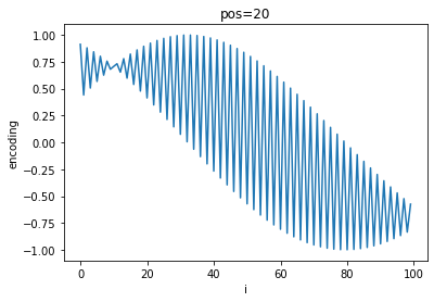
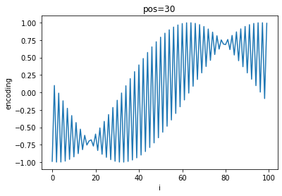
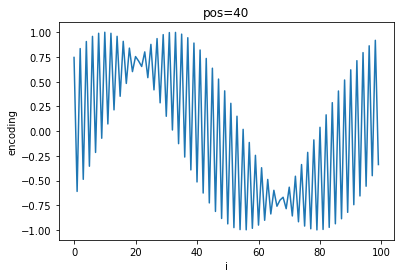
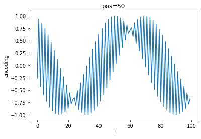
As $pos$ increases, a general sinusoidal shape appears on top of the high-frequency oscillations and shifts to the left while the frequency of oscillation between each $i$ increases.

A matrix of shape (num_words, embedding_len) can now be created using $PE$. $i$ ranges from $0$ to embedding_len$-1$ and $pos$ ranges from $0$ to num_words$-1$. This matrix of positional encoding values is simply added elementwise to each embedded sequence matrix to create positionally-encoded inputs.

Here's an implementation that includes a more explicit example of what I'm talking about:

Encoder

The encoder is the stack of functions in the left rectangle of the transformer diagram. The encoder takes in an embedded and positionally-encoded input sequence and produces an output called the context. Keeping with our translation example, the encoder context will be a matrix where each row contains encoded information corresponding to each of the input vectors. The encoder has several parts, each explained below.

I. Multi-head attention and $Q$, $K$, $V$

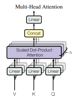
The multi-head attention layer takes in 3 inputs, labeled $Q$ (query), $K$ (key), and $V$ (value). The diagram provided in the paper is a bit misleading as it doesn't explicity say that $Q$, $K$, and $V$ are created by passing the encoder input through 3 different linear layers (1 layer for each $Q$, $K$, $V$). Also note that the provided diagram shows an additional dimension for the $Q$, $K$, and $V$ layers. This is the head dimension $h$ and will be discussed later. For now, let's just consider how the encoder input is used to generate $Q$, $K$, $V$ with a single head ($h=1$).

Recall from the previous section that the our example input to the encoder is an embedded, positionally-encoded matrix representing a sentence. I'll refer to this input as enc_inp with shape (num_tokens, embedding_len). Here's my simplified version of the multi-head attention diagram (this is technically a single-head attention diagram):

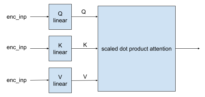
In this diagram, there is only $h=1$ head. So, there is no need for a concatenation layer because that layer is used to join the scaled dot product attention outputs across multiple heads. To use multiple heads, imagine creating a stack of these single-head attention layers. The diagram provided in the paper helps with this visualization.

To implement this functionality, it's much simpler (and more efficient) to increase the output dimensions of the $Q$, $K$, $V$ linear layers than it is to create and track $h$ layers individually.

To clarify, let's consider the $h=1$ case. A single enc_inp matrix has dimensions (num_tokens, embedding_len). This is the input shape to each $Q$, $K$, $V$ layer. The $Q$, $K$, $V$ layers are used to transform the input into a new representation. The paper keeps the same shape, so with $h=1$, $Q$, $K$, $V$ each take an input with shape (num_tokens, embedding_len) and produce an output with shape (num_tokens, embedding_len).

Now let's consider the $h=2$ case. The input shape to the $Q$, $K$, $V$ layers is still (num_tokens, embedding_len). Each head layer takes in the same input. A single head layer produces an output with shape (num_tokens, embedding_len), as described above. Now that we have 2 head layers, we get 2 output matrices with shape (num_tokens, embedding_len). Since these matrices have the same number of columns, you can combine them into one big matrix with shape (2 * num_tokens, embedding_len). This is the same as saying the shape is ($h$ * num_tokens, embedding_len).

Now, each $Q$, $K$, $V$ layer can be modified to accept an input of shape (num_tokens, embedding_len) and produce an output with shape ($h$ * num_tokens, embedding_len). This method only requires the definition of single $Q$, $K$, $V$ layers. Notice that it also doesn't require any concatenation as the paper's diagram suggests since the output matrices of the $Q$, $K$, $V$ layers are already "concatenated." If this isn't clear, manually work through an example with $h=2$. First compute the outputs for each head layer individually, and then see how the exact same output is created when the $Q$, $K$, $V$ layers just produce a larger output.

II. Scaled dot product attention

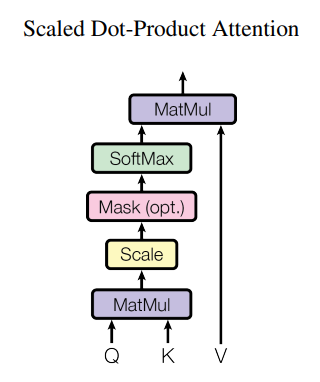
The scaled dot product attention function is composed of a few relatively straightforward operations. This is where the "attention" (the only thing we need, apparently) is mathematically implemented. It is expressed with the equation:

The mask operation will be described and used later in the decoder section of this writeup. It is not needed for the encoder. In more informal language, the encoder attention is computed by doing the following:

1. matrix multiply $Q$ by the transpose of $K$ -> store result in variable $a$
2. divide $a$ by the square root of embedding_len (scale step) -> $a$
3. compute softmax across each row of $a$ -> $a$
4. matrix multiply $a$ by $V$ -> $a$

This series of operations gives you an output that has the same shape as the input $Q$, $K$, $V$ matrices.

III. Attention intuition

The implementation of the attention function is easy enough. But why is it this set of operations and why is it all we need?

Understanding attention begins with understanding what the $Q$, $K$, and $V$ linear layers produce. The $Q$, $K$, $V$ layers each transform enc_inp into some new representation that has the same shape as enc_inp. Each of these layers ideally learns to produce a meaningful transformation during the training process. The $Q$ layer is expected to learn to capture the relationship between each token with all other tokens in the sequence. The $K$ layer is expected to capture which tokens in the sequence are relevant to the current token. The $V$ layer is expected to learn how to capture meaningful content in the sequence. These learning expectations are still a bit unclear to me and are not entirely intuitive, but this high-level understanding of $Q$, $K$, $V$ is enough to move forwards.

The first step of computing attention is to matrix multiply $Q$ and $K$, and then scale the result by the square root of embedding_len (called $d_k$ in the paper). This step can be thought of as combining and averaging the information contained in $Q$ and $K$.

For example, let's consider a matrix $Q$ with shape (3, 2) and a matrix $K$ with shape (3, 2). In order to do this matrix multiplication, $K$ must be transposed to have a shape (2, 3).

The matrix multiplication operation consists of computing the dot products between the rows of $Q$ and the columns of $K$.

Each row in the result of the matmul represents a combination of the information in that row of $Q$ with each column of $K$.

Next, this result is scaled by the square root of the number of columns in $Q$. I've assumed that $Q$, $K$, and $V$ will all have the same shape and that shape will be the same as a single input matrix that has the shape (num_tokens, embedding_len). So, in this example, $d_k=$ embedding_len $=$ 2. Why divide by the $\sqrt{2}$ instead of just $2$? Dividing by the square root of $d_k$ gives the resultant matrix a variance of $1$, which is important for keeping the values within a reasonable range.

$QK^T$ is now operated on by softmax. Softmax scales each row such that its values sum to 1. Elements greater in value before the softmax are transformed into values closer to 1, while lesser values are transformed into values closer to 0.

Effectively, we have combined the information contained in $Q$ with the information contained in $K$, scaled that combined information, and finally scaled that combined information into weights between 0 and 1. These weights can be thought of as the "attention weights." Next, these weights are combined with the information contained in $V$ with a matmul. Similar to before, the resultant rows of this matmul will contain the information in the corresponding row of $V$ with each set of attention weights. The final output of this scaled dot product attention function will be weighted towards the values that require more attention in $V$.

IV. The finished encoder

After the attention is calculated for each head, the results are combined with a concatenation step. This step can be avoided by combining all heads of $Q$, $K$, and $V$ into larger matrices, as described earlier. The results are passed through a linear layer to get the final values of attention. The original encoder inputs, enc_inp, are now added to each head of attention values. This result is then normalized. This is accomplished using Pytorch's Layernorm(). After this, the result is passed into a simple feed forward network that contains a linear layer with ReLU and a linear layer after that. This result is then added to the output of the previous add & norm step, and then passed through another Layernorm(). This last output of the encoder is the context. It will be passed on to the decoder.

Okay, great, we have an encoder. But there's one more thing: the encoder block in the architecture diagram has "Nx" next to it. The paper says to use a stack of N encoders, where each encoder's input is the previous encoder's output (except for the first encoder, whose input is enc_inp), and the encoder context is the final output of the encoder stack. Visually, this looks like:

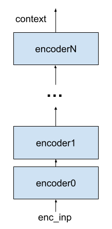
The output of the final encoder in the stack is the context. For reference, the paper uses a stack of N=6.

Here's my implementation of a single encoder described in this section (note the additional dimension in the input to accomodate for training in batches and also note that embedding_len = input_size and note the added logic for dropout during training):

Decoder

The decoder is the stack of functions in the right rectangle in the transformer architecture diagram. During training, the decoder will take in an embedded and positionally-encoded target sequence (the spanish sentence in our example) and the context produced by the encoder. During inference (after the model is trained), the target sequence is not available, and the sequence prediction must be made one token at a time.

I. Masked multi-head attention

The decoder consists of the same parts as the encoder, except there is a masking step in its first attention layer. The masking step prevents each token in the target sequence from accessing information about future tokens.

To understand what masking does and why it's needed, let's look at how a prediction is made after the transformer model has been trained. Let's use the example from earlier where the input to the encoder is the english sentence "He is tall." and the input to the decoder is the spanish sentence "El es alto."

We first embed and positionally encode the english sentence to produce its numeric matrix representation. This matrix is passed through the entire stack of encoders to produce the encoder context. The input to the decoder is the target output and the encoder context. We don't have the target spanish sentence yet, so we must predict it token-by-token. In this first inference step, the input to the decoder will just contain the special token "<S>" and no other data. We pad the decoder input with rows of 0s (just like we did with the encoder input) to give it the correct dimensions. The data is passed through the decoder, and a sequence of predicted outputs are produced. We want to predict the first word in the target sequence, so we are only interested in the first predicted output of this sequence. Let's assume it correctly predicts "El" as the first token in the target sequence. Now we update the decoder's input with the newly-predicted token, and then go through the same process to predict the second token. The decoder now recieves an input of ["<S>", "El"] and the encoder context remains unchanged. The decoder input is once again padded with rows of 0s to get the correct dimensions, and the data is passed through the decoder to get the next prediction. This process continues until the special token "<E>" is the next prediction in the sequence or when the maximum number of tokens have been predicted. The predicted sequence consists of each token that was predicted in each step of inference. This process of iteratively producing predictions token-by-token must now be reflected in training.

We could format our training data and structure our training code in a way to follow the same iterative sequence generation as used during inference, but that would be quite inefficient and rather silly of us since we already have the entire target sequence available during training. We can save a lot of compute with masking.

As described in the Attention intuition section above, when $Q$ is multiplied by $K^T$, each row in the resultant matrix contains the information of a row in $Q$ combined with the information in each column of $K$. When you consider that $Q$ and $K$ will contain a numeric representation of the tokens in the target sequence, you see that each row in the resultant matrix contains the information of a token in $Q$ multiplied by each token in $K$. Informally, let's say that a linear transformation performed by the $Q$, $K$, $V$ dense layers on a token t can be represented by $Q_d(\text{t})$, $K_d(\text{t})$, $V_d(\text{t})$, respectively. The multiplication can be thought of like:

Note that I didn't show all of the columns in the resultant matrix above. The representation above is conceptual and doesn't represent the actual operations that occur, but I think it's a good visual to imagine the scenario at hand. To reiterate one more time, the rows in $QK^T$ contain the information of a token in $Q$ combined with the information of each token in $K$.

When the transformer predicts the first token, it should only have access to the information pertaining to the value "<S>". So, we want to 0 out any results in $QK^T$ that contain information on any of the other tokens in the sequence. On the first step of inference, we want:

When the transformer predicts the second token, it should only have access to the information pertaining to the values "<S>" and "El". Again, we want to 0 out any other results in $QK^T$.

For the third token, it's the same deal:

Hopefully, you're starting to see the pattern. With each additional token, the corresponding row in $QK^T$ adds another column. If you extend this pattern, you get a matrix with a lower triangle of data. During training, the entire target sequence is available, which means that each row in $QK^T$ will not be zeroed in the appropriate locations. The demonstration above suggests that we should get these 0s after the $QK^T$ operation, but that is not what we actually do. First, we compute $QK^T$ (without zeroing anything out), and we later zero out the appropriate positions in the softmax step. The example of $QK^T$ above is just for conceptual clarification. The actual sequence of operations to zero out future information looks like:

Since $\lim_{x\to-\infty} e^{x} =0$, softmax outputs 0 for large negative values. We can take advantage of this to zero out unwanted values. We simply set the upper triangle of $QK^T$ to large negative values. This masking scheme will allow us to pass an entire target sequence into the decoder during training instead of going token-by-token. The 0s in each row prevent the information of future tokens in the sequence from leaking into tokens earlier in the sequence. This propagates all the way to the final predicted outputs.

II. The rest of the decoder

The masked multi-head attention layer outputs are added with the decoder inputs and passed through a LayerNorm(). The output of this layer becomes the input to the $Q$ linear layer in the next attention layer. The inputs to the $K$ and $V$ linear layers for this attention layer are both the encoder context. This attention layer combines these three pieces of information, as described already. The rest of the operations in the decoder are shown in the transformer architecture diagram and have already been explained in the encoder section.

In code, the whole decoder looks like (note that I again added an optional line to apply dropout during training):

The finished transformer

All pieces of the transformer have been discussed. The only work remaining is to put together the stack of encoders and decoders and pass their output into a few more simple layers shown in the architecture diagram. A forward pass looks a bit different depending on if we are in training or performing inference. During training, we will pass data through the stack of encoders and the stack of decoders. During inference, we will create the encoder context a single time and then only pass data through the decoder. In the code below, I have implemented a full transformer using the encoder and decoder classes previously shown. The forward pass in this transformer class is only for training, the code for inference will be presented in a second writeup that details training the model because it is a bit more specific to the modeling task (or maybe I'm just lazy and don't want to refactor).

For the english-spanish translation example, the output of our transformer is a matrix where each row has the length of the entire spanish vocabularly used in the training data and each value is a softmax probability where that value's index maps to a token in the vocabulary. So, if there are 20,000 unique spanish tokens in our input training data, each row will have a length of 20,000, and the value at each index is the model's predicted probability for that token to be correct. The maximum probability of each row is found and the index is mapped back to the spanish vocabulary to get the actual predicted token.

Concluding remarks

The transformer architecture is not totally intuitive to me, but at a certain point, I'm not sure how intuitive it is to anyone. Honestly, why this specific set of matrix operations leads to successful sequence-to-sequence predictions is beyond me. But, I have shown that it does in part 2 (oh and I guess a bunch of other people have too, but ya know, I had to check that they weren't lying).